Working with libreoffice. Guidelines for practical work “Tabular processor Libreoffice Calc. Working in the spreadsheet processor Libreoffice Calc. Using tools to speed up data entry

MINISTRY OF EDUCATION AND SCIENCE OF THE RUSSIAN FEDERATION

FEDERAL STATE BUDGET EDUCATIONAL

HIGHER EDUCATION INSTITUTION

"TULA STATE UNIVERSITY"

Institute of Applied Mathematics and Computer Science

Department of Information Security

COMPUTER SCIENCE

METHODOLOGICAL INSTRUCTIONS

for laboratory work

for full-time students in the field of study (specialty)

090303 (10.05.03) “Information security of automated systems”

Introduction. Work order

Previously, before the start of the laboratory lesson, students get acquainted with the goals and objectives of the laboratory work, with the work assignment, and also study the explanations set out in the “Theoretical Information” paragraph of the guidelines for performing the next work.

During the lesson, students complete the task (see paragraphs “work assignment”) in the sequence set out in paragraph “Procedure for completing the work.” For most jobs, tasks are performed according to individual options. The option is assigned by the teacher conducting the lesson.

Based on the results of the work, a report on the implementation of laboratory work is drawn up. Requirements for the report are specified in the guidelines for each work. The report is first completed electronically (during class), then printed for the next lesson.

Every laboratory work requires protection. For protection, the student must present: the result of completing the assignment (general and in his own version), a report in electronic form and in paper. During the defense of the work, the student is asked questions about the progress of the assignments or about the theoretical material discussed in the work. If the student gives satisfactory answers to all questions, the work is considered protected and the teacher puts the appropriate number of points (from 0 to 3) and his signature on the title page of the report.

Laboratory work 1. Text editor MS WORD. General operating principles.

Purpose and objectives of the work

This work studies the basic principles and techniques of working in the MS Word text editor.

THEORETICAL INFORMATION

Launch MS Word. To launch MS Word via button Start you need to do the following: move the mouse to the button Start and press the left key; select the item from the list that appears Programs; click on the menu item - Microsoft Word.

In this operating mode, the MS Word editor starts with the creation of a new document. Figure 1 shows the general view of the MS Word window (depending on the version of MS Word, the window view may be different).

Menu item – File. When you click on the File button, a drop-down menu appears with the following items:

- "Create"– Creates a new MS Word file (Ctrl-N);

- “Open”– Opens a dialog box in which you are prompted to select a file to work with (Ctrl-O);

- “Close”– Closes the working file;

- "Page settings"– Opens a dialog box with page parameters;

- "Preview"– Opens a document window, which shows the appearance of the document when printed on a printer;

- "Seal"– Opens the document print dialog box.

- "Properties"– Opens a window containing information about the working document.

- "Exit"– closes the MS Word application. If, when you click on exit, the document is not saved, a menu appears asking you to save the document.

This menu also shows a list of the last few documents you worked with. When you click on them, they open in the editor.

Configuring document page parameters. To configure document settings, click – Menu→File→Page Setup, after which the window shown in Figure 2 will open.

Bookmarked “Fields” customizable: margin values ​​(top, left, bottom, right and binding); document orientation (portrait and landscape); type of document on the page – “Pages”; scope of application of page parameters in relation to the document.

Bookmarked “Paper Size”: Select paper size from the list; the exact paper size is set; The scope of application of page parameters in relation to the document is determined.

Bookmarked “Paper Source” configured: rules for starting a new section; rules for differentiating headers and footers; scope of application of page parameters in relation to the document.

Menu item – Edit. When you press the button Edit, the menu shown in Figure 3 opens.

Actions:

- "Cancel"– actions are canceled according to the stack principle,
(Ctrl-Z);

- "Repeat"– repeats the last action (Ctrl-Y);

- "Cut out"– deletes the selected fragment and places it in the buffer,
(Ctrl-X);

- "Copy"– copies the selected fragment to the buffer, (Ctrl-C);

- "Insert"– inserts information from the buffer into the document (Ctrl-V);

- "Select all"– selects the entire contents of the document (Ctrl-A);

Menu item – View. When you click on a menu item View The menu shown in Figure 4 opens.

This window allows you to configure the presentation of the document on the screen.

Menu item – Window. When you click on a menu item Window The menu shown in Figure 5 opens.

Actions:

- "New"– opens the current document in a new window;

- “Arrange everything”– distributes all open MS Word windows on the computer screen;

- "Divide"– allows you to split the screen into several work areas containing open documents in MS Word.

Menu item – Help. When you open this menu, a list of items appears containing reference information and various assistants in working with MS Word.

Setting up MS Word.

MS Word panels are configured through the Tools→Settings menu item. After clicking on this item, a window with settings opens, Figure 6. The window contains bookmarks: toolbars, commands and parameters.

The “Toolbars” tab specifies which panels should be on the screen. The “Commands” tab specifies which commands should be on the screen. The “Parameters” tab contains additional parameters for panel properties.

Inserting objects.

Inserting objects into MS Word is done through the Insert→Object menu. A window appears on the screen with two tabs: Create and Create from file. When selected from the “Create” section, a new object is added to the document, and when clicked from the “Create from file” item, it is already added from an existing object/file. See Figure 7.

WORK TASK

Recall the basic capabilities of a word processor (Microsoft Word) for creating simple documents. Create a report electronically.

Making a report

The work report is prepared in electronic and paper form.

The report must contain: a title page, the purpose and objectives of the work, the work assignment, the results of the task (according to your own version). A sample title page is presented in the appendix to these guidelines.

PROCEDURE FOR PERFORMANCE OF THE WORK

1. Launch MS Word and create a new file. Start writing your lab report. The title page (sample) is presented in the appendix to these guidelines. Type the text of the title page of the work report (individual for each student) and save the file on disk. Open the file from disk and configure the MS Word page settings to the following parameters (paper size - A4; page orientation - portrait; Margins (left - 2.5 cm; right -1.5 cm; top - 2 cm; bottom - 2 cm))

2. Get acquainted with the material presented in the “Theoretical information” paragraph in practice, remember the hot keys of the main commands.

3. Configure the panels. Display the panels - Standard and Formatting. Become familiar with a functional set of commands, such as the fonts, kerning, and text alignment commands.

4. Insert “Microsoft Equation 3.0” objects. Type the formulas according to your choice. Bring a list of notations to the formula, for example, like this:

5. Insert the “Microsoft Word Picture” object. Create a drawing explaining the formulas (the drawing must be created independently, and not inserted ready-made, for example, from the Internet). Label the drawing as - Figure 1 – Description of the drawing. Create multiple drawings if necessary

Task options

Var. No.	Description of the formula
	Relations connecting the lengths of the sides of a right triangle with the degree measure of angles (via sine and cosine)
	Relations for determining the area of ​​a trapezoid, the area of ​​a parallelogram and the area of ​​a rhombus.
	Cosine theorem and sine theorem
	Pythagorean theorem, calculating heights in a right triangle.
	Calculation of the area of ​​a triangle (at least two formulas)
	Calculation of the area of ​​a quadrilateral (at least two formulas)
	Finding the radius of the inscribed and circumscribed circle (for a triangle)
	Height of the pyramid, volume of the pyramid.
	Volume of a cone, surface area of ​​a cone.
	The volume of a cylinder is the surface area of ​​the cylinder.
	Relations between trigonometric functions of one argument (at least three formulas)
	Equation of a straight line on a plane (at least two options)
	The distance from a point to a line in a plane, from a point to a plane in space, the distance between two lines in space.

Laboratory work 2. Word processor OpenOffice (LibreOffice) Writer. Interface OpenOffice Writer

Purpose and objectives of the work

This work studies the basic principles and techniques of working in the OpenOffice (LibreOffice) Writer text editor.

THEORETICAL INFORMATION

The main workspace of the Writer text editor is shown in Figure 1.

Writer includes several context-sensitive toolbars that, by default, appear to float in response to the current cursor or selection position. For example, when the cursor is in a table, the floating Table toolbar appears, and when the cursor is in a numbered or bulleted list, the Bullets and Numbering toolbar appears.

To show or hide rulers, you must select View > Ruler .

The status bar displays the following information:

· current page number and total number of pages in the document. Double-clicking the left mouse button on this window opens a navigator with which you can navigate through the document. Right-clicking displays all bookmarks in the document;

· current page style. Double-clicking the left mouse button opens the page settings formatting window. Right-clicking allows you to select a style from a pop-up list;

· display scale. Right-clicking allows you to select a different scale from the list;

· display the current typing mode– insertion or replacement;

· display current selection mode– standard, extended or add mode;

· hyperlink mode allows you to transfer them from the active state to the change mode;

· sign of saving changes. If changes made to the document have not been saved, an asterisk (*) symbol will be displayed in this window;

· digital signature window. With it, you can add or remove a digital signature to a document (right-click);

MINISTRY OF EDUCATION AND SCIENCE OF THE RUSSIAN FEDERATION Federal state budgetary educational institution of higher education

vocational education

TOMSK STATE UNIVERSITY OF CONTROL SYSTEMS AND RADIO ELECTRONICS

DEPARTMENT OF AUTOMATED CONTROL SYSTEMS

Laboratory workshop for the course “Informatics and Programming”

developer Ph.D., associate professor of the Department of Automated Control Systems

Sukhanov A.Ya.

Sukhanov A.Ya.

Computer science and programming: Training manual for laboratory work – 226 p.

The educational manual contains the program and tasks for laboratory classes, as well as all the necessary forms of documents for completing the tasks.

(c) Sukhanov A.Ya., 2010

1 Laboratory work No. 1. LibreOffice................................................... ...............................................
1.1.Launch LibreOffice Writer.................................................... ........................................................ ...............
1.2.Entering text.................................................... ........................................................ ....................................
1.3.Text formatting.................................................... ........................................................ ................
1.4.Saving a document.................................................... ........................................................ ...............
1.5.Using toolbars.................................................... ........................................
1.6.Adding new features to the toolbar.................................................... .........
1.7.Editing text.................................................... ........................................................ ................
1.8.Page settings.................................................... ........................................................ ...............
1.9.Design of paragraphs (Paragraphs)................................................... ........................................................ .
1.10.Sections and breaks.................................................... ........................................................ .......
1.12.Inserting a picture into text.................................................... ........................................................ ..............
1.13.Formulas................................................... ........................................................ ...................................
1.14.Styles and formatting.................................................... ........................................................ ..........
1.15..AutoCorrect and AutoCorrect options.................................................... .........................................
1.16.Task................................................... ........................................................ ......................................
2 Learning LibreOffice Writer macros.................................................... ...................................................
2.1.Objects and classes. ........................................................ ........................................................ ...............
2.2.Variables and objects in Basic.................................................... ........................................................ .....
2.3.Basic operators.................................................... ........................................................ ...........................
2.4.Procedures and functions. ........................................................ ........................................................ ..........
2.5.Creating a macro in LibreOffice.................................................... ........................................................ ...
2.6.Tasks LibreOffice Writer macros.................................................... ...........................................
3 Laboratory No. 2 Studying LibreOffice Calc spreadsheets.................................................... .....
3.1.General information about the Calc spreadsheet in LibreOffice....................................................
3.2.Spreadsheet structure.................................................... ........................................................
3.3.Construction of diagrams.................................................... ........................................................ .............
3.4.Task 1. .................................................... ........................................................ ....................................
3.5.Task 2. ................................................. ........................................................ ....................................
4 Laboratory work No. 3 Using Calc as a database, studying macros...................
4.1.Data filtering.................................................... ........................................................ ...................
4.2. Pivot tables. ........................................................ ........................................................ ...............
4.3. Total fields and grouping............................................................ ........................................................ .....
4.4.Study Calc macros Basic................................................ ........................................................
4.4.1 Calculation of bonuses based on interest.................................................... ...............................
4.4.2 Accrual of bonuses. Using the function. ........................................................ ..
4.4.3 Calculation of formulas, implementation of computational functions. ......................................
5 Laboratory work No. 4 Study operating system MS-DOS and working in the command line
line........................................................ ........................................................ ........................................................ .
5.2.What is an operating system?.................................................. ........................................................
5.3.DOS operating system.................................................... ........................................................ ........
5.4.What is meant by a file. ........................................................ ........................................................
5.5.ASSIGNMENT................................................... ........................................................ ...................................
6 Laboratory work No. 5 Study of the operating room Windows systems and Far shells...............
6.1. Appearance of Far................................................... ........................................................ ...........................
6.2.Basic Far manager commands.................................................... ........................................................ ..
6.3.Working with panels.................................................... ........................................................ ........................

6.5.Viewing the contents of the disc.................................................... ........................................................ .....
6.6.Sorting the list of files.................................................... ........................................................ ..........
6.7.Launch programs.................................................... ........................................................ ...........................
6.8.Creating folders.................................................... ........................................................ ............................
6.9.Viewing the folder tree.................................................... ........................................................ ................
6.10.Copying files.................................................... ........................................................ .............
6.11.Deleting files.................................................... ........................................................ .......................
6.12.Working with multiple files.................................................... ........................................................ .
6.13.Searching files.................................................... ........................................................ ............................
6.14.Quick file search.................................................... ........................................................ ................
6.15.Creating text files.................................................... ........................................................ ......
6.16.Viewing text files.................................................... ........................................................ .....
6.17.Editing text files.................................................... ...........................................
6.18.Quick view mode.................................................... ........................................................ .......
6.19.Folder search.................................................... ........................................................ ...............................
6.20.Using a filter.................................................... ........................................................ ............
6.21.Changing file attributes.................................................... ........................................................ ...
6.22.User command menu.................................................... ........................................................ ......
6.23.Determination of Far actions depending on the file name extension..................................
6.24.Working with the FTP client.................................................... ........................................................ ...............
7 Studying the Windows operating system. ........................................................ ................................
8 Explore Forms and visual controls in OpenOffice or LibreOffice. ...............
8.1.Learning msgbox.................................................... ........................................................ ........................
8.2.Creating a Dialog Box with an Input Line. ........................................................ ....................
8.3.Creating a dialogue.................................................... ........................................................ ........................
8.4.Implementation of a dialogue with a button.................................................... ........................................................ ...
8.5.Object model.................................................... ........................................................ ........................
8.6.Studying Forms and Controls.................................................... ....................................
8.7. Study of flags. ........................................................ ........................................................ ...............
8.8. Study of Switches. ........................................................ ........................................................ .
8.9.Text fields.................................................... ........................................................ ...........................
8.10.List................................................... ........................................................ ....................................
8.11.Combo box.................................................... ........................................................ ......................
8.12.Macro implementing the use of a text field and lists....................................................
8.13.Element Counter.................................................... ........................................................ ....................
8.14.Independent task.................................................... ........................................................ ......
9 Learning Java................................................... ........................................................ ........................................
9.1.Three principles of OOP.................................................... ........................................................ ....................
9.2.Implementation of the program in Java.................................................... ........................................................ ..
9.3.Using NetBeans.................................................... ........................................................ ..........
9.4.What are interfaces.................................................... ........................................................ ................
9.5.Swing system.................................................... ........................................................ ...........................
9.5.1 Japplet class.................................................... ........................................................ .......................
9.5.2 Icons and labels.................................................... ........................................................ ....................
9.5.3 Text fields.................................................... ........................................................ ...............
9.5.4 Buttons................................................... ........................................................ ...............................
9.5.5 JButton class.................................................... ........................................................ ......................
9.5.6 Checkboxes.................................................... ........................................................ ...............................
9.5.7 Switches.................................................... ........................................................ ...............
9.5.8 Combo fields............................................................ ........................................................ ...............
9.5.9 Tabbed panels.................................................... ........................................................ ..........
9.5.10 Scroll bars.................................................... ........................................................ ............

10 Applications - Help with the first and second labs, learning Writer and Calc. ........................................................ ........................................................ ................................171

10.1.LibreOffice.................................................... ........................................................ ...............................
10.1.1 Launching LibreOffice Writer.................................................... ........................................................ .
10.1.2 Entering text.................................................... ........................................................ .......................
10.1.3 Editing text.................................................... ........................................................ ...................
10.1.4 Text formatting.................................................... ........................................................ ...
10.1.5 Saving a document.................................................... ........................................................ ....
10.1.6 Using toolbars.................................................... ............................
10.1.7 Adding new features to the toolbar....................................................
10.1.8 Editing text.................................................... ........................................................ ....
10.1.9 Page settings.................................................... ........................................................ .......
10.1.10 Formatting Paragraphs.................................................. ....................................
10.1.11 Sections and breaks.................................................... ...........................................
10.1.13. Inserting a picture into text.............................................................. ...............................................
10.1.14. Formulas........................................................ ........................................................ ...................
10.1.15 Styles and formatting.................................................... ...................................................
10.1.16 Task.................................................... ........................................................ ...........................
10.2.Learning LibreOffice Calc spreadsheets.................................................... .......................
10.2.1 General information about the Calc spreadsheet in LibreOffice....................................
10.2.2 Spreadsheet structure.................................................... ............................................
10.2.3 Constructing diagrams.................................................... ........................................................ ..........
10.2.4 Task 1. ................................................. ........................................................ ...............................
10.2.5 Task 2. ................................................. ........................................................ ...............................

1 Laboratory work No. 1. LibreOffice

LibreOffice Writer is a word processor designed for creating, viewing and editing text documents, with the ability to use the simplest forms of algorithms in the form of macros. LibreOffice is a free, independent, open source office suite developed by The Document Foundation as an offshoot of OpenOffice.org, which includes the Writer word processor. Quite detailed information about the LibreOffice package can be found at http://help.libreoffice.org/Writer/Welcome_to_the_Writer_Help/ru.

Any word processor is an application computer program designed for the production, including operations of typing, editing, formatting, printing, any type of printed information. Sometimes a word processor is called a text editor of the second kind.

In the 1970s - 1980s, word processors were machines designed for typing and printing texts for individual and office use, consisting of a keyboard, a built-in computer for simple text editing, and an electrical printing device. Later, the name "word processor" was used for computer programs intended for similar uses. Word processors, unlike text editors, have more opportunities for formatting text, introducing graphics, formulas, tables and other objects into it. Therefore, they can be used not only for typing texts, but also for creating various kinds of documents, including official ones. Word processing programs can also be divided into simple word processors, powerful word processors, and publishing systems.

1.1. Launching LibreOffice Writer

First of all, you need to launch LibreOffice Writer.

IN Depending on the operating system used, for example, Linux or Windows, you need to follow the following algorithm, in many ways it is the same for the specified operating systems:

IN Start menu (Windows) select Programs + LibreOffice and launch WordProcessor LibreOffice Writer or Office LibreOffice, in the graphical shell of KDE or GNOME Linux you can select the Application Launcher menu and in the Applications submenu Office and LibreOffice. When you select LibreOffice, a window for creating LibreOffice documents will open (Figure 1), among which are Writer documents; in the specified window, Writer documents are marked as Text Document. When you select WordProcessor LibreOffice Writer, a window with a blank document form will immediately open (Figure 2).

Figure 1 - LibreOffice

Figure 2 - Window with a LibreOffice Writer document

1.2. Entering text

The main component of LibreOffice Writer documents: letters, notes, posters, business papers - is usually text. Type some text into the new Writer document that opens when you launch the program.

1 . Enter some sentence.

2. Press the Enter key.

To switch from the Russian keyboard layout to the English one, you need to press the Ctrl+Shift or Alt+Shift keys - depending on Windows settings or Linux. The keyboard indicator appears in the taskbar next to the clock. You can switch layout

also using the mouse. To do this, left-click on the indicator and select the desired layout from the menu that appears. To delete the character to the left of the cursor (the flickering vertical bar), press Backspace. To delete the character to the right of the cursor, press the Delete key.

Editing Text After you initially enter text, you will likely need to edit it. Let's

Let's try adding and then removing text in the document. The cursor shows where in the document characters entered from the keyboard will appear. Left-click once in the document to change the cursor position. The cursor can also be moved using the arrow keys.

By default, Writer works in insert mode. This means that as you type, all text to the right of the cursor moves to make room for new text.

4. Double click on some word.

5. Press the Delete key.

The existing text will move back and fill the empty space.

1.3. Text formatting

1. Left-click on the page margin.

2. Click on Symbols on the menu bar.

3. Select the Font tab.

4. From the Family list, select a font called Liberation Serif.

5. In the Style list, select Bold.

6. Use the scroll bar to scroll through the Size list and select a value

7. In the Font Effects area, check the Shadow box.

8. Click OK.

9. Click anywhere in the document to deselect text.

In addition, you can compact the font; this is done, for example, so that the text occupies a certain number of pages or a certain volume, if suddenly the resulting volume is larger than the required one (Tab Position and Spacing, select sparse or compacted (Scale Width)).

The same page of character options can be selected from the Format menu.

You can also format paragraph and page options separately, and you can also select them from the Format menu. Page and paragraph options are discussed next.

1.4. Saving a document

Documents must be saved. The frequency of saving a document corresponds to the time that you do not mind spending on restoring data lost in the event of a computer failure.

2. Select the Save command. The Save As dialog box appears, shown in Figure 3. Writer automatically suggests a name for the document (usually Untitled 1). Enter any other name

Figure 3 - LibreOffice (KDE) file save window

3. In the File name (name) text box, enter a name for the file.

4. The text you enter will replace the text selected in the File name (name) field.

5. Additionally, you can also use the Backspace keys to delete text here

and Delete.

6. Expand the Folder (Save in) list at the top of the dialog window.

7. Select any of your drives or folders.

Let's say you decide to add a couple more words to your document. How can I open it again?

1. Select File from the menu bar.

2. Select the Open command.

3. Select a drive. Expand the list of Folders and files.

4. Click your folder icon.

5. Select your document icon

6. Click the Open button.

Toolbars provide access to some of the most commonly used menu commands. If you are better with a mouse than a keyboard, you will be more comfortable using toolbars.

Figure 4 - View of toolbars

Displaying the toolbar on the screen Word contains many toolbars, which usually group buttons related to a large topic, such as Tables and Borders, Drawing, Database, and Web. .

They can be displayed and removed from the screen as needed.

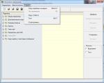
1. Right-click on any toolbar or menu bar and select Customize Toolbar. A drop-down list of all panels will appear on the screen

A spreadsheet is a rectangular matrix consisting of cells, each of which has its own number.

LibreOffice Calc is designed to work with data tables, primarily numeric.
Creating workbooks
LibreOffice Calc window

The LibreOffice Calc working window is shown in Fig. 1.

Rice. 1. LibreOffice Calc working window

The default LibreOffice Calc document is named "Untitled 1". Consists of several sheets (3 by default) with a standard ODS extension. At the user's request, the number of sheets can be increased.
The worksheet consists of rows and columns. Columns are numbered from A to AMG, and rows from 1 to 1048576. Cell addresses are formed from the column number and row number (for example, A1). Cells are accessed by their addresses.
Operations with sheets:

• renaming – double click on the sheet name on its label or “Rename” in the shortcut context menu;
• deletion – menu “Edit” → “Sheet” → “Delete sheet” or “Delete” of the shortcut context menu;
• moving or copying – menu “Edit” → “Sheet” → “Move / copy sheet” or the corresponding item in the shortcut context menu. To copy, you need to check the “Copy” checkbox in the “Move / copy sheet” window;
• adding - click on the shortcut of the sheet in front of which a new sheet is inserted, in the context menu of the shortcut select the item “Add sheets” (Fig. 2)

Rice. 2. Insert Sheet Dialog Box
In this dialog box, specify the position, name of the sheet, quantity and click the “OK” button. The Insert Sheet dialog box can also be accessed from the Insert → Sheet menu.
If the book consists of a large number of sheets and all the labels are not visible, then you should use the arrows located to the left of the labels.
Selecting cells and ranges(+ arrows or left mouse button; – different areas). All cells in a row or column can be selected by clicking on the row or column header. To select a worksheet in the current workbook, you need to click on the worksheet tab. To select all cells of a worksheet, you need to click on the button for selecting the entire sheet (the rectangle at the intersection of the row and column headings) or press the keyboard shortcut.
Entering data into a worksheet
Worksheet cells can contain text, constants, and formulas. You cannot perform mathematical calculations on text data. By default, numeric data is right-aligned and text is left-aligned. If the category name does not fit in width, then the right cell (if it is not empty) overlaps the next one. The width of columns can be changed using the Format → Column → Width menu (you can use the Optimum Width command) or manually by dragging the borders in the column header row. If data has been typed but not yet entered, corrections can be made directly in the cell and in the formula bar.
After the data has been entered, to correct it you need to go to editing mode. To do this, double-click on the desired cell. A insertion pointer appears in the cell. After editing is completed, the entry of new data must be confirmed by pressing a key. Clicking cancels the changes made.
Data types.
The type determines the amount of memory allocated for data and possible operations with it. Let's describe the main data types of LibreOffice Calc.
Whole numbers– these are numbers that are divisible by one without a remainder: 4; -235. Numbers in parentheses are treated as negative.
Real number or whatever they call it real number is any positive number, negative number or zero. For example, 24.45 (separator is comma).
Fractions: 7/8; 4/123.
To enter percentages, type the % symbol after the number. If the entered number is a monetary value, then rubles are typed at the end. (rubles).
If the entered numeric constant does not fit the width of the cell, it is displayed on the screen as ####. In this case, the column width must be increased.
date and time. You can enter a date, for example, September 21, 2011, by typing 09/21/11 on the keyboard.
The time is entered as 13:21 or 14:15:00.
Formulas. All formulas in LibreOffice Calc must begin with the symbol = . To capture your input, the formula appears in the cell and in the formula bar. After pressing the key, the value calculated by the formula will appear in the cell, and the input line will be cleared.
When calculating a value using a formula, the expressions inside the parentheses are evaluated first. If there are no parentheses, the operations are as follows:

• function values ​​are calculated;
• operation of exponentiation (operation sign ^);
• multiplication and division operations (operation signs *, /);
• operations of addition and subtraction (operation signs +, -).

The formula can contain numbers, links (cell addresses), and functions as operands.
Examples of formulas: = 4*8^4-12; B2+SIN (1.576).
The value of a formula depends on the contents of the referenced cells, and it changes when the contents of those cells change.
For view formula argument values On the worksheet, you need to double-click the left mouse button on the cell with the formula. In this case, the arguments in the formula and the corresponding values ​​on the worksheet are highlighted in the same color (Fig. 3)


Rice. 3. View formula argument values
Operations at the same level are performed from left to right. In addition to these operations, communication operations are used in arithmetic expressions:
: range;
; Union;
! intersection.
The & sign (ampersant) is used to combine texts.
Function is a predetermined formula. A function has a name and arguments enclosed in parentheses. Arguments are separated from each other by the symbol “;”. You can use other functions (if they operate on the same data type), constants, cell addresses, and cell ranges as arguments.
A range is a group of cells that form a rectangle. A range is indicated by a cell in the upper left corner of the rectangle and a cell in the lower right corner of the rectangle. For example, the designation C5:F9 describes the range of cells located at the intersection of rows numbered 5, 6, 7, 8, 9 and columns C, D, E, F.
For example, SUM(A3;E1:E4) – this function has two arguments. The first is A3, the second is E1:E4. The numbers in cells A3, E1, E2, E3, E4 are summed.
Formula bar after selecting the “Function” operator (sign “ = " on the formula bar) contains the following elements: a drop-down list of recently used functions, a "Function Wizard" button, a "Cancel" button, an "Apply" button and an input line (Fig. 4).


Rice. 4. Formula bar
Entering formulas. Formulas can be entered in several ways: using icons, entering from the keyboard, or both methods at the same time.
1. Click the cell where you want to paste the formula.
2. Click the Function icon (the " sign = ") in the formula bar. An equal sign will appear in the input line, and you can now enter the formula. The formula can be entered using the “Function Wizard”, selecting the necessary operators from the drop-down list and entering actions from the keyboard.
3. After entering the desired values, press the key or the Accept button to paste the result into the current cell. If you need to clear the input line, press the key or the Cancel button.
You can enter values ​​and formulas directly into cells, even if the input cursor is not visible. All formulas must begin with an equal sign.
You can also press the “+” or “-” key on the numeric keypad to start entering a formula. NumLock mode must be on. For example, press the following keys in sequence: +50 - 8 .
The cell displays the result 42. The cell contains the formula =+50-8.
Set of functions using the "Function Wizard". Button " Function Wizard" on the toolbar looks like f ( x ) .
Built-in functions allow you to perform the necessary calculations quickly and easily. LibreOffice Calc has over 350 functions. In the event that none of the built-in functions are suitable for solving the task at hand, the user has the opportunity to create his own (custom) function.
For ease of use, functions are grouped into categories: database; date Time; financial; information; brain teaser; mathematical; arrays; statistical; spreadsheets; text; additional.
When you click this button, the wizard starts working. You can select a function from the category you need. For example, to calculate the hyperbolic arc cosine of a number, select cell E41, click on the “Function Wizard” button, select the “Mathematical” category, and the “ACOSH” function. On the right side of the dialog box, a description of this function is provided (Fig. 5).


Rice. 5. Function Wizard Dialog Box
To use this function, you must click the “Next” button or double-click on the “ACOSH” function on the left side of the dialog box. You can also manually enter a formula in the input line according to the example given after the function name on the right side of the dialog box.
After clicking the “Next” button or double-clicking on the “ACOSH” function, the dialog box will take the following form (Fig. 6)


Rice. 6. Selecting the “ACOSH” function
In this window, you can enter a number from the keyboard in the “Number” field. At the top it is indicated what value this number can take. When you click on the “Select” button, an input line appears (Fig. 7), into which you can enter the name of the cell that contains the number to be calculated (the cell can also be selected directly on the worksheet by selecting it with the left mouse button).

Rice. 7. Number selection
After selecting the required cell, you must click on the button
In this case, we return to our dialog box, where the result is already displayed (Fig. 8)


Rice. 8. “Function Wizard” after selecting a cell containing a number
In the “Structure” tab, the “Function Wizard” shows us the structure of this operation, the degree of nesting (Fig. 9)


Rice. 9. Tab "Structure"
We press the button. The result of this function is written to cell E41 (Fig. 10).


Rice. 10. Result of the function
LibreOffice Calc can work with both individual cells and data arrays.
Addressing
LibreOffice Calc distinguishes between two types of cell addressing: absolute and relative. Both types can be applied in one link and create a mixed link.
Relative link is perceived by the program as indicating a route to the addressed cell from the cell containing the formula. When copying a formula, the relative links will be changed so that the route will be preserved. Relative links are used by default in Calc.
Absolute link specifies the absolute coordinates of the cell. When you copy a formula, the absolute cell reference will not change. An absolute reference is specified by specifying a dollar sign before the row and column number, for example $A$1.
A mixed reference is a combination of absolute and relative references when both a row and a column are different ways addressing, for example $A4, B$3. When you copy a formula, the absolute part of the link does not change.
You can set a link when entering a formula directly by entering from the keyboard or by pointing (mouse clicking on the desired cell).
Often in formulas you need to specify references to a range of cells. Calc uses three address operators to specify a range:
range operator (colon): the reference addresses all cells located between two specified cells, for example, =SUM(A1:B2) - returns the sum of the values ​​of cells A1, A2, B1 and B2;
range join operator (semicolon): the reference spans the cells of the specified individual ranges, for example, =SUM(A3;E1:E4) - returns the sum of cells A3, E1, E2, E3, E4;
range intersection operator (exclamation mark): the reference covers the cells included in each of the specified ranges, for example, =SUM(B2:D2!C1:D3) - returns the sum of cells C2 and D2.
Creating Rows
Scheme for entering the same value or formula into part of a column or row:
1. enter a value or formula into a cell and click;
2. Place the mouse pointer on the cell fill marker and drag it in the desired direction while holding down the left key.
The cell fill marker is a small rectangle in the lower right corner of the cell:

Scheme for entering numerical values ​​by regression type:
1. enter the first two elements of the progression into two adjacent cells;
2. select these cells;
3. Place the mouse pointer on the fill marker of the selected cells and drag it in the desired direction while holding down the left mouse button.

Formatting
Data stored in cells can be displayed in one of several formats. You can select the data presentation format and cell design method in the “Format Cells” dialog box (Fig. 11). You can call it by pressing a keyboard shortcut, selecting the “Cells...” item in the “Format” menu or the “Format Cells...” item after right-clicking on a cell (calling up the context menu).
Formatting includes the following elements:
- setting the number format;
- choice of fonts;
- drawing frames;
- filling cells with color and pattern;
- data alignment;
- data protection.


Rice. 11. Format Cells Dialog Box
The “Format Cells” window contains several tabs, which you can navigate between by clicking on the tab tab. Brief description of the tabs:
Numbers– allows you to select one of the ways of presenting data with the ability to refine it (right). For example, for the Numeric format, you can specify the number of decimal places. In this case, an example of the selected data representation is displayed in the field on the right.
Font– the tab controls the choice of font (style, style, size, language).
Font effects– allows you to set the color, overline, underline, relief, outline, shadow of the font.
Alignment– a bookmark allows you to control the way text is placed in a cell, text rotation in a cell, and word wrapping in a cell.
Framing– the tab allows you to create a frame around cells using borders of different styles and thicknesses.
Background– the tab controls the cell fill color.
Cell protection– the tab controls the protection of cells from changes.

Error values ​​when calculating using formulas

Error value	Error code	Explanation of the error
		The column is too narrow to display the full contents of the cell. To solve this problem, increase the column width or use the Format → Column → Optimal Width menu.
		The operator or argument is not valid.
		The calculation resulted in a certain range of values ​​being overflowed.
		A formula within a cell returns a value that does not match the definition of the formula or the functions used. This error may also mean that the cell referenced by the formula contains text rather than a number.
		A formula within a cell uses references that do not exist.
		Identifier cannot be evaluated: no valid reference, no valid domain name, no column/row, no macro, invalid decimal separator, padding not found.
		Division by 0 is specified.

Tracking cell relationships.
In large spreadsheets, it can be difficult to determine which cells are used for complex formula calculations, or which cell formulas a given cell participates in.
LibreOffice Calc allows you to use a visual graphical representation of the relationships between cells. The cells that are used for formula calculations are called “influencing cells.” Cells that use the active cell in their formulas are called "dependent cells."
To trace influencing and dependent cells, you can use the menu command “Tools” → “Dependencies”. The menu of this service is shown in Fig. 12.

Rice. 12. Dependencies menu
Influential cells. This function displays relationships between the current cell that contains a formula and the cells used in that formula. For example, the operation of adding two cells (A1 and A3). The result of the addition (formula “=A1+A3”) is written in cell C2. To view the cells that influence C2, select this cell and use the “Influencing Cells” service. At the same time, LibreOffice Calc will use arrows to indicate the cells that affect cell C2 (Fig. 13)

Rice. 13. Influential cells
Remove arrows to influencing cells. Removes one level of arrows to influence cells inserted using the Influence Cells command.
Dependent cells. This command draws arrows to the active cell from formulas that depend on the values ​​in the active cell. Let's use the previous example, but now select cell A1 and see that cell C2 depends on cell A1 (Fig. 14)

Rice. 14. Dependent cells
Remove arrows from dependent cells. Removes one level of arrows from dependent cells inserted using the Dependent Cells command.
Remove all arrows. Removes all dependency arrows contained in the spreadsheet.
Source of error. This command draws arrows to all influencing cells that cause an error in the selected cell.
Circle the incorrect information. When you call this command, all cells in the worksheet that contain values ​​that do not meet the validation rules are marked.
Update arrows. This command causes all arrows on the sheet to be regenerated, taking into account changes in formulas since the last time the dependencies were placed.
Update automatically. Automatically update all dependencies in a worksheet whenever the formula changes.
Fill mode. This command enables dependency filling mode. The mouse cursor turns into a special symbol and can be used to click on any cell to view the dependencies of the influencing cells. To exit this mode, press the key or click the Exit Fill Mode command in the context menu.
Merging cells – To merge two or more cells, you need to select the cells and click the button on the Formatting panel “Merge and Center Cells” or use the menu “Format” → “Merge Cells”. These operators can also be used when splitting cells.

Creating Charts
LibreOffice allows you to graphically display data in the form of a chart to visually compare data series and see their trends. Charts can be inserted into spreadsheets, text documents, drawings, and presentations.
Charts in LibreOffice Calc are created using the Chart Wizard. Before activating it, it is advisable to select the data that will be used in the chart, although this can be done during the construction of the chart.
The selected area should contain cells with the names of rows and columns that will be used as category names and legend text. You can use data in non-contiguous areas to build a chart. Data series can be added to the source table, and the table itself can be placed in the chart area. The “Chart Wizard” is called from the main menu using the command “Insert” → “Diagram” (Fig. 15) or the button on the toolbar.


Rice. 15. "Chart Wizard"

Working with the Chart Wizard requires sequential completion of four steps:
1. Selecting the chart type and view (bar chart, bar chart, pie chart, area chart, line chart, XY chart, bubble chart, grid chart, stock chart, column chart, and line chart).
2. Specifying the range of data to be displayed on the chart and choosing the orientation of the data (data series are defined in the rows or columns of the table); chart preview.
3. Set up data ranges for each series.
4. Chart design: adding a legend, naming the chart and axes, applying markings.

Editing charts
Once the diagram is created, it can be modified. The changes concern both the type of diagrams and its individual elements. Range of chart editing options:
1. Click on the diagram to change the properties of objects: size and position on the current page; alignment, dough transfer, outer boundaries, etc.
2. To switch to the chart editing mode, double-click on the chart with the left mouse button: chart data values ​​(for charts with their own data); chart type, axes, titles, walls, grid, etc.
3. Double-click a chart element in chart editing mode: To change the scale, type, color, and other parameters, double-click an axis.
Double-click a data point to select and change the data rad that the point belongs to.
Select a data series, click it, and then double-click a data point to change the properties of that point (for example, a single value in a histogram).
Double-click the legend to select and edit it. Click and then double-click a symbol in the selected legend to change the corresponding data series.
To change properties, double-click any other chart element, or click the element and open the Format menu.
4. To exit the current editing mode, click outside the diagram.
Also, to select chart elements, you can use the “Chart Formatting” toolbar, which appears after double-clicking on the chart (Fig. 16)


Rice. 16. Chart Formatting Toolbar
Using this panel, you can select chart elements in the drop-down list, view the format of the selected element (the “Selection Format” button) and make the necessary changes. This panel also contains the following buttons:

Panel view	Properties
	Chart type
	Show/hide horizontal grid
	Show/hide legend
	Text scale
	Automatic marking

To add elements to the diagram, you must use the “Insert” menu (Fig. 17) and select the required element (you must first select the diagram by double-clicking the left mouse button).

Rice. 17. Insert menu
“Headings” – you can add or change the title of the title, subtitle, the name of the X, Y, Z axes, and additional axes. To move an element, you need to select it and drag it to the desired location. You can also delete a selected title using the Legend key. The legend displays the labels from the first row or column, or from the range that was specified in the Data Series dialog box. If the chart does not contain a label, the legend will display text as "Row 1, Row 2..." or "Column A, Column B..." according to the row number or column letter of the chart data. It is not possible to enter text directly; it is generated automatically based on the name of the cell range. Using the “Insert” → “Legend” menu, you can change its location or hide it. “Axes” tab. Makes it possible to add missing axes to the diagram. “Grid” – provides the insertion of a grid into the diagram, which improves perception. Removing grid lines is achieved by unchecking the corresponding checkboxes. Formatting the diagram area is reduced to changing the appearance (frame and fill) (Fig. 18).

Rice. 18. Chart Area Dialog Box

Managing the 3D view of charts. To control the three-dimensional appearance of diagrams, LibreOffice Calc provides the ability to change the viewing angle of the diagram by changing three special parameters: perspective, appearance and lighting (Fig. 19)

Rice. 19. 3D view
This feature is included in the “Format” → “3D Image” command.
Sorting lists and ranges
LibreOffice Calc introduces different types of data sorting. You can sort rows or columns in ascending or descending order (text data in alphabetical or reverse alphabetical order). In addition, LibreOffice Calc allows you to create your own sort order. The “Sorting” dialog box (Fig. 20) is called up using the “Data” → “Sorting” menu. In this case, you must first select the columns, rows, or simply the data that needs to be sorted.

Rice. 20. Sort Dialog Box
You can also sort data using the buttons on the Standard toolbar.

Applying filters to analyze lists. Filters allow you to place the results of queries based on criteria into a separate table, which can be used for further processing. Filter a list means hiding list rows except those that meet the specified selection criteria.
Using AutoFilter. Before using an autofilter, you need to select the data (maybe the entire header row) that you want to filter. Menu “Data” → “Filter” → “Autofilter”. For each column header, LibreOffice Calc will set an autofilter in the form of an arrow button. As a result of the autofilter, LibreOffice Calc displays the filtered rows.
Using a standard filter. It is also very convenient to use the standard filter, which makes it possible to use a variety of criteria associated with the logical functions AND or OR. Calling a standard filter – menu “Data” → “Filter” → “Standard filter” (Fig. 21)


Rice. 21. Standard Filter Dialog Box
The standard filter can also be used when the AutoFilter is applied.

Using the advanced filter(Data → Filter → Advanced Filter). Select a named area or enter a range of cells that contains the filter criteria you want to use.
Data forms. When performing database-specific operations such as searching, sorting, summarizing, LibreOffice Calc automatically treats the table as a database. When viewing, changing, deleting a record in the database, as well as when searching for records by a specific criterion, it is convenient to use data forms. When you use the Data → Form command, LibreOffice Calc reads the data and creates a data form dialog box (Figure 22).

Rice. 22. Data Form Dialog Box
In the data form, one record is displayed on the screen, it is possible to view subsequent records and create a new one. When you enter or change data in the fields of this window, the contents of the corresponding database cells change (after entering new data, you must press a key).
Selection of parameter. In the case of the parameter selection function, we are talking about a simple form of data analysis of the “what if” type, that is, it is necessary to select a value of the argument at which the function accepts set value. In particular, the fit function can be used to find the root of a nonlinear equation. The target cell's value is the result of the formula. This formula refers directly or indirectly to one or more influencing cells. The fit function changes the value of the influencing cell so as to obtain the specified value in the target cell. The influencing cell itself can also contain a formula.
To use the parameter selection function, you need to select the cell with the target value and select the “Tools” → “Parameter selection” command (Fig. 23).


Rice. 23. Dialog box “Parameter Selection”

Target Cell—In the cell containing the formula, enter a reference to the cell containing the formula. It contains a link to the current cell. In the case presented in Fig. 12, the target cell contains the squaring formula. Click another cell on the worksheet to link it to the text box.
Target value– here you indicate the value that you want to get as a new result. Let's say we need to figure out what number needs to be squared to get the value 121. Accordingly, we enter “121” as the target value.
Changing a cell - here you specify a link to the cell containing the value that you want to adjust to select the value.
After entering the settings, click “OK” and LibreOffice Calc offers us the option to replace the cell (Fig. 24). The result of our actions is the number 11.

Letter from the Department of Education and Science of the region dated November 20, 2019 No. 1.01-29/5522 “On monitoring the level of informatization of organizations in the regional education system for 2019” (TOGBU without image process)

Lesson #1
Topic: Spreadsheets. Purpose. Spreadsheets LibreOffice Calc
Cells and cell ranges. Data entry and editing.
Entering formulas.

Spreadsheets

Spreadsheets (ET)– these are special programs designed to work with data in tabular form:

To perform calculations on data,

To build charts based on tabular data,

To sort and search data based on a specific criterion,

To conduct data analysis and calculate “what if?” scenarios,

To create databases,

For printing tables and their graphical representation.

The first ETs appeared in 1979.

The generally recognized ancestor of spreadsheets as a separate class of software is Dan Bricklin, which together with Bob Frankston developed the program VisiCalc in 1979. This computer spreadsheet Apple II became very popular, turning the personal computer from a toy for technophiles into a mainstream business tool.

Purpose.

ETs are intended for economists, accountants, engineers, scientists - all those who have to work with large amounts of numerical information.

3. LibreOffice Calc

LibreOffice Calc - , included inLibreOffice. With its help, you can analyze the input data, do calculations, make forecasts, summarize data from different sheets and tables, build charts and graphs. In addition to this program in the packageLibreOfficeincludes other office programs.

Office suiteLibreOfficecan be freely installed and used in schools, offices, universities, home computers, government, budgetary and commercial organizations and institutions in Russia and the CIS countries according to .

Package contents LibreOffice

Module

Notes

LibreOffice Writer

LibreOffice Calc

LibreOffice Impress

Training program

LibreOffice Base

Mechanism for connecting to external and built-in DBMS

LibreOffice Draw

LibreOffice Math

Screen view

The screen view is standard for WINDOWS applications :

A title bar that contains the name of the program and the current document.

Menu bar with basic commands.

Toolbars – Standard, Formatting and Formula Bar.

A working field that consists of cells. Each cell has its own address: the name of the column and the row number at the intersection of which it is located. For example: A1, C8, P15. There are only 256 columns (last IV), 65636 rows.

There are scroll bars on the left and bottom of the screen. To the left of the bottom scroll bar are tabs with worksheet titles. Thus, we see only a piece of a huge table that is formed in the PC memory.

DocumentationLibreOffice Calc

Documents that are created using LibreOffice Calc, are called workbooks and have an extension . O.D.S. . The new workbook has three worksheets called SHEET1, SHEET2 and SHEET3. These names are located on the sheet labels at the bottom of the screen. To move to another sheet, click on the name of that sheet. The worksheet may contain

data tables,

charts (as a table element or on a separate sheet).

Actions with worksheets:

Rename a worksheet. Place the mouse pointer on the spine of the worksheet and double-click the left key or call the context menu and select the command rename.

Inserting a worksheet. Select the sheet tab in front of which you want to insert a new sheet, Insert  Sheet, or using the context menu.

Deleting a worksheet. Select the sheet tab, Edit Delete, or using the context menu.

Move and copy a worksheet. Select the sheet tab and drag it to the desired location (with the CTRL key pressed - copy) or via the clipboard.

Cells and cell ranges.

The work field consists of rows and columns. Rows are numbered from 1 to 65536. Columns are designated with Latin letters: A, B, C, ..., AA, AB, ..., IV, total - 256. At the intersection of the row and column there is a cell. Each cell has an address consisting of a column name and a cell number. The cell address is written only in English - this is important

To work with several cells, it is convenient to combine them into “ranges”.

A range is cells arranged in a rectangle. For example, A3, A4, A5, B3, B4, B5. To write a range, use " : ": A3:B5

Examples: A1:C4, B6:E12, G8:H10

Exercise:

- select the following ranges of cellsB 2: D 7; A 1: G 2; D 4: H 8

- write down ranges

7 . Data entry and editing.

IN LibreOffice Calc You can enter the following types of data:

• Text (for example, headings and explanatory material).

  Functions (eg sum, sine, root).

Data is entered into cells. To enter data, the required cell must be highlighted. There are two ways to enter data:

Just click in the cell and type the required data.

Click in the cell and in the formula bar and enter data in the formula bar.

Press ENTER.

Changing data.

Select a cell  press F 2  change data.

Select a cell  click in the formula bar and change the data there.

To change formulas, you can only use the second method.

Entering formulas.

A formula is an arithmetic or logical expression used to perform calculations in a table. Formulas consist of cell references, operation symbols, and functions. LibreOffice Calc has a very large set of built-in functions. With their help, you can calculate the sum or arithmetic average of values ​​from a certain range of cells, calculate interest on deposits, etc.

Entering formulas always begins with an equal sign. After entering a formula, the calculation result appears in the corresponding cell, and the formula itself can be seen in the formula bar.

Action

Examples

Addition

Subtraction

Multiplication

A1/B5

Exponentiation

A4^3

=, <,>,<=,>=,<>

Relationship signs

You can use parentheses in formulas to change the order of operations.

Exercise:

Enter the following data

Make sure the active font is English.

Place the table cursor in cell D2.

Left-click in the formula bar.

Enter the equal sign and then the formula: B2*C2. Press the key<Enter>.

Verify that a numeric value appears in cell D2

Exercise:

Fill out the following table, in the “amount” field write down the formulas for calculating the total amount

Lesson #2
Topic: Autocomplete spreadsheet cells.
Autofill cells with formulas. Using the Sum function

1. Autocomplete.

A very convenient tool is autofilling adjacent cells. For example, you need to enter the names of the months of the year in a column or row. This can be done manually. But there is much more convenient way:

Enter the desired month in the first cell, for example January.

Select this cell. In the lower right corner of the selection frame there is a small square - a fill marker.

Move the mouse pointer to the fill marker (it will look like a cross), while holding down the left mouse button, drag the marker in the desired direction. In this case, the current value of the cell will be visible next to the frame.

If you need to fill out some number series, then you need to enter the first two numbers into the adjacent two cells (for example, enter 1 in A4, and 2 in B4), select these two cells and drag them by the marker (from the lower right corner of the second cell) the selection area to the desired size.

Exercise:

- using autocomplete to build rows

- from 1 to 50,

- from 2 to 100,

- January December

Autocomplete formulas

Construction of the simplest data series is possible using the method described above. If the dependence is more complex, then the formula is used as the initial value of the range.

Example: There is a legend about the inventor of chess, who asked as a reward for his invention as much grain as would be produced if 1 grain was placed on the first square of the chessboard, 2 on the second, 4 on the third, 8 on the fourth, etc., that is each next one is 2 times more than the previous one. There are 64 squares on the chessboard.

For the first cell - 1 grain

On the next one – 2, i.e. twice as much, but instead of the number 2 in cell B 2 we enter the formula. Since the pattern is described by the equation y =2x, the formula will be similar =A 1*2

Press Enter and stretch the second cell by the marker down by 64 cells

Let's now calculate the sum of all cells in the example. To do this, select the required range (in our case from 1 to 64 cells (A 1 – A 64)). Find the “amount” button at the top and click on it

The amount value will be written in the next cell in order. If the amount value should be in a separate cell, then you need to activate this cell, click on the amount icon, select a range and press “ enter".

Exercise:

- find the sum of all natural numbers from 1 to 100 inclusive

- find the sum of all odd numbers from 1 to 99

- find the sum of squares of natural numbers from 1 to 10 (1 2 + 2 2 +3 2 +…)

Lesson #3
Topic: Relative and absolute addressing

The spreadsheet may contain both basic(original), and derivatives(calculated) data. The advantage of spreadsheets is that they allow you to organize the automatic calculation of derived data. For this purpose, in table cells use formulas. Moreover, if the source data changes, the derived data also changes.

In cell D 3 we create a formula that calculates the sum of the numbers in cells B 2 and C2

If you now change the data, for example, in cell B 2, the sum value will be automatically recalculated

Let's now try to copy the formula down using the drag-and-drop method.

Please note that after copying the formula to another cell, its appearance has changed, i.e. instead of links to cells B 2 and C 2, there are links to cells B 3 and C 3.

This method is called relative addressing. It is convenient to use when filling out the same type of data.

However, there are situations when using this method leads to incorrect calculations. Let's look at an example:

Let's say we need to transfer money from dollars to rubles; the current dollar exchange rate is written in one of the cells

In other cells, enter the amount in dollars

Let's create a formula in cell B 3 to convert dollars to rubles

P Let's try copying the formula to the lower cells

We see that the result was calculated incorrectly (it should turn out not 0 but 1200 and 3000)

A careful study of the resulting formula shows that cell A 3 has “turned” into cell A 4 (which is correct, since the value “40” is now substituted), but the second factor has now automatically become the cell below cell C 2 - cell C 3, in which it is empty, and, therefore, the second factor becomes the number 0. This means that for the result to be correct, it is necessary to fix the second cell in some way, preventing its entry from being changed.

This can be done using so-called absolute addressing. The essence of this method is that in writing the formula, a $ sign is placed before the letter or number, which prevents the corresponding letter or number from changing. If this sign appears before both the letter and the number, then we are dealing with absolute addressing, and if only before a letter or only before a number - with mixed addressing(in this case, some of the formula links may change when copied)

Let's change our initial formula using the absolute addressing method

And copy it down

Please note that part of the formula that is enclosed in “dollars” has not changed!

We will demonstrate the method of absolute and mixed references using the example of compiling a multiplication table

You can fill all the table cells with formulas manually; it is easier to do this using autofill, although you should be careful here, since the links are shifted when copied.

Let's try to simply copy the formula in cell B 2 down

As you can see, the result, as one would expect, is incorrect. Let's try to understand what's going on by analyzing the formula, for example in cell B 3

Correctly it should be =A 3*B 1, which means the number “1” located in the formula in cell B 2 must be “fixed”

Let's now try to copy the formula down

Now everything is calculated correctly, note that the number on the right side of the formula has not changed

Exercise:

Make a 10 x 10 multiplication table

-

Lesson #4
Subject: Standard features in LibreOffice Calc

1. Standard features.

Calculations that the program allows you to makeCalc, are not limited to the simplest arithmetic operations. It is possible to use a large number of built-in standard functions and perform very complex calculations.Functions In OpenOffice.org, Calc refers to combining multiple computational operations to solve a specific problem. The values ​​that are used to evaluate functions are calledarguments . The values ​​returned by functions as a response are calledresults .

When we start entering a formula (by pressing the “=” key), the Name field in the formula bar is replaced by a drop-down list of standard functions.

This list contains the ten most recently used functions, as well as More Functions, which opens the Function Wizard dialog box.

This dialog box allows you to select any of the standard functions available in Calc.

· financial (functions for calculating various economic indicators, such as rate of return, depreciation, rate of return, etc.);

· date and time (using the date and time functions, you can solve almost any problem related to date or time, in particular, determining age, calculating length of service, determining the number of working days in any period of time, for example: TODAY() - enters the current date of the computer) ;

· mathematical (functions for performing various arithmetic and algebraic operations, for example: ABS() - returns the modulus of a number, SUM() - summing a range of cells, SQRT() - square root value, etc.);

· statistical (this category contains various functions that work with such branches of mathematics as probability theory, mathematical statistics, combinatorics);

· text (using text functions, it is possible to process text: extract characters, find the ones you need, write characters to a strictly defined place in the text, and much more, for example: LOWEL() - makes all letters in a line of text lowercase);

· brain teaser (these functions help create complex formulas that, depending on the fulfillment of certain conditions, will perform various types of data processing or perform branching calculations, for example: IF(), AND(), OR()).

When you select a function, a brief description of it appears, so you can easily find the function you need. At first, mathematical and logical functions will be enough for you.

Formulas and functions can also be entered manually by simply typing their names in the formula bar.

If a function appears at the very beginning of a formula, it must be preceded by an equal sign, as in any other formula. Remember that when writing a function, there must be opening and closing brackets, and you should not insert spaces between the function name and the brackets.

For example, if cell A5 contains a formula with the exponentiation function =POWER(A 4;3), the value of that cell will be the value of A4 raised to the power of 3.

In the future we will often refer tomathematical functions, to which include such functions known from school mathematics courses asSIN() - sine, COS() - cosine, TAN() - tangent, LN() - natural logarithm, SQRT() - square root of a number, etc.

Let's look at an example:

You need to find the largest value of a range of cells. Without using the function, such a calculation is impossible. Below is a function that allows you to find the largest value in a range of cells:

MAX(A1:A10), where

MAX – function for determining the largest value;

A1:A10 – range of cells among which you want to find the largest value.

As another example, consider constructing a table of values ​​of some function on a given interval and with a given step.

Let's make a table of values ​​of the sine function in the interval from 1 to 2 with a step of 0.1

First, we construct a series of values ​​for the independent argument ( x), taking into account the specified parameters

In cell B 2 insert the sine function (by any method) from the argument of cell A 2

Copy the formula down

The result is ready!

Exercise:

Make a table of values ​​of the cosine function on the interval from 1 to 3 with a step of 0.2

Create a table of function values y = x 2 in the range from 0 to 3 in increments of 0.1

Lesson #5
Topic: “Using logical functions.
Building graphs and diagrams"

1.Logic Functions FunctionIF

The IF function is used to check conditions in calculations.

Recording format:

IF (log_expression; value_if_true; value_if_false)

A logical expression is any value or expression that evaluates to TRUE or FALSE. For example, A10=100 is a Boolean expression; if the value in cell A10 is 100, then the expression evaluates to TRUE. Otherwise - FALSE.

The table calculates the salary of each employee, it is determined by salary (the same for everyone) and length of service (different)

The coefficient is calculated as follows:

If Experience >= 10 years, then it is equal to 2, otherwise – 1.

In column E we insert the following formula: =IF (C2>=10;2;1),

Accordingly, in column F: =D2*E2

In the same example, we will calculate the coefficient as follows:

Experience up to 10 years – 1,

From 10 to 20 – 1.5,

Therefore, here you need to choose from 3 options. We use nested functions IF.

In column E we insert the formula: =IF (C2<10;1;IF (C2>=20;2;1,5))

Please note that in the formula the second IF is inside parentheses

The table will look like:

2. Diagramming

LibreOffice calc provides ample opportunities for creating business graphics - charts and graphs. They display data more clearly than numbers in table cells. By looking at charts or graphs, you can immediately analyze the data in the table.

Diagram is a graphical representation of data in a table.

Diagrams are built on the basis of ready-made tables.

Graphs and diagrams are built using diagram wizards

Chart Wizard is a series of dialog boxes that allow you to create a new diagram or edit an existing one.

In dialog box No. 1, select the chart type.

In dialog box No. 2, you can specify the range of data on which the chart will be built.

The Rows or Columns radio buttons allow you to select the direction of the data to plot when the selected range is a rectangular area.

Data series– sets of data presented graphically as bars, sectors or lines on a chart.

In dialog box No. 4, the chart parameters are set.

Elements common to all types:

TITLE – You can enter a title for the chart.

Legend– an area in which colors and patterns corresponding to certain data in the diagram are deciphered. For a legend to have meaningful labels, it is necessary to highlight the numeric data along with the row and column headings in the table.

DATA LABEL – numerical, percentage or text labels next to each chart element.

DATA TABLE – a fragment of the source table with data for the diagram is placed under the diagram.

Construction order:

Enter the original data set (collection of cells)

Select the desired range (in the simplest case, one column or row)

Click the diagram button

In the wizard that opens, determine the structure of the future diagram or graph step by step

In more complex cases, another (or several) column with text (or data) is added to the diagram, which in the diagram is converted into labels of rows, columns, sectors, etc.

Please note that a ready-made chart can be edited by changing the data, chart color, labels, legend, etc.

Exercise:

draw up a chart of the cost of products purchased in a store using the following template, calculate the total cost yourself, highlight only columns B and E (via the key ctrl )

3. Graphing

As an example, consider the procedure for constructing a graph of a function y = sin (x ) in the range from 0 to 6.3 in increments of 0.1

1) Preparing the initial data

2
) Select the entire data range and call the chart wizard

3) At the first step of the wizard, select the following items:

4) You can click the “Done” button. The schedule is ready!

Exercise :

Graph the function y = x 2 in the range from -3 to 3 in increments of 0.1

Plot the function cos ( x /2 ) in the range from -1 to 4 with steps of 0.1

Lesson #6
Topic: "Spreadsheets - as a means of computer modeling"

Our model, which we will develop based on ET, will be biological rhythms.

What are biological rhythms?

We all live according to certain laws. There is a theory that human life is subject to three cyclical processes called biorhythms. Strictly speaking scientifically, biorhythms are periodically repeating changes in the nature and intensity of biological processes and phenomena in a living organism. These are the cyclical phenomena occurring in nature reflected by the body. A simpler and more well-known concept is the “biological clock”. The Greek physician Herophilus (300 BC) discovered that the pulse of a healthy person changes throughout the day. Subconsciously, a person chooses the time when it is easier for him to work. Approximately 400 - 500 years ago, people began to live by the clock, and before that there was no need for them, since natural and biological clocks worked. The body's biorhythms - daily, monthly, annual - have remained virtually unchanged since primitive times and cannot keep up with the rhythms of modern life.

In recent years, the theory of “three rhythms” has gained wide popularity. The triggering mechanism for these exceptional rhythms is only the moment of human birth. A person was born, and rhythms arose with a period of 23, 28 and 33 days, determining the level of his physical, emotional and intellectual activity.

Physical biorhythm characterizes a person’s vitality, i.e. his physical condition.

Emotional biorhythm characterizes a person’s internal mood, his excitability, and the ability to emotionally perceive the environment.

The third biorhythm characterizes the thinking abilities and intellectual state of a person.

Graphic representation these rhythms is sine wave. Many believe that the “ups” of the graph, which is a sinusoidal dependence, correspond to more favorable days. One-day periods in which phase switching occurs (“zero” points on the graph) and which are supposedly characterized by a decrease in the corresponding level of activity are called “critical days,” i.e. unfavorable. If two or three sinusoids cross the same “zero” point at the same time, then such “double” or “triple” critical days are especially dangerous. Moreover, in some countries, on such days, people in risky professions (pilots, stuntmen, etc.) are given a day off.

According to the theory of biorhythms, the capabilities of the human body change periodically. After a certain number of days (period), the body returns to the same state.

There are several cycles of the body: physical, intellectual, emotional.

This does not depend on the age, gender, or nationality of the person.

The beginning of each biorhythm coincides with the date of birth.

It is known that:

The physical cycle lasts 23 days,

Emotional – 28 days,

Intellectual – 33 days.

Let's start creating a model of biological rhythms

1) Creation of a mathematical model:

These cycles can be described by the following expressions, in which the variable x is the number of days lived by a person:

Physical cycle PHYS(x) = sin(2pi x/23)

Emotional cycle EMO(x) = sin(2pi x/28)

Intelligent cycle INT (x) = sin(2pi x/33)

It is clear that all these functions periodically change their values ​​from -1 to 1 (function range sin (x ) ).

Knowing how many days have passed since a person’s birthday, you can easily calculate the value of the above functions for the current day. To track changes in functions you need x increase by the required number of days.

Having a table of function values, you can build its graph, which makes it easy to track its appearance.

To find out how many days have passed since your birthday, you need to subtract the date of birth from the current date

The final formula will look like

Sin (2 (T k -T 0)/k), where

T 0 – date of birth of a person

Tk – settlement date

K – cycle period

It makes sense to construct all 3 function graphs corresponding to each cycle in one coordinate system

2) Drawing up a computer model

Let's fill out the table:

In cell A1, enter the column name - Date of Birth

In B1 we enter – Settlement date

In C1 we enter - Physical cycle

In D 1 we enter – Emotional cycle

In E1 we enter – Intelligent cycle

The table header is ready.

Data input.

In A2 – the person’s date of birth, for example 01/01/2000

In B2 – the calculated date, for example 02/19/2004

In C2, the formula for determining the physical cycle = sin (2*pi()*(B2-A2)/23)

In D 2, the formula for determining the emotional cycle = sin (2*pi()*(B2-A2)/28)

In E2, the formula for determining the intelligent cycle = sin (2*pi()*(B2-A2)/33)

As of today, the data has been received. Let's enter several estimated dates, for example, a week ahead from the current date. To do this, copy the calculated date down to the required position value

All that remains is to copy down the formulas for the cycles. True, you need to be careful here, since one of the links (try to guess which one yourself!) is fixed and, therefore, the formulas need to be modified.

The final graph might look something like this:

Exercise:

Try expanding the scope of the schedule by extending the date forward to 1 month. Plot the resulting graphs

3) Analysis of simulation results.

Look at the resulting graphs. The higher the sine wave rises, the higher the corresponding abilities and vice versa. Exceptions may be those days in which the graph crosses the X-axis. Then the abilities can be unpredictable: either wonderful or very bad.

Exercise:

1. After analyzing the diagram, select “unfavorable” days for physical education

2.Choose days when answers in lessons will be the most (least) successful.

3.Check your mood when your emotional biorhythm indicators are on the decline or on the rise on your chart.